"On the server I never knew where my electricity came from. On the phone I can feel the battery I am draining and the warmth I am adding to someone's pocket. It has made me a more considerate model."
An Image Classifier Newly Aware of Its Power Budget
At the edge, watts and milliwatt-hours are as hard a constraint as accuracy, and a model that ignores them does not ship; the design problem is to deliver the most accuracy per joule and per byte on a chip you do not control. This section takes the compressed, compiled model of the previous two sections to the devices where most vision actually runs: embedded modules like the NVIDIA Jetson family, and the phones in billions of pockets through runtimes like Core ML, TensorFlow Lite, and ExecuTorch. It also covers the architectures, the MobileNet and EfficientNet families, that were designed for these budgets from the first layer rather than compressed into them after the fact. The camera-and-sensor pipeline of Chapter 1 is now the front end of a system you must fit into a power envelope.
The cloud is comfortable: effectively unlimited power, abundant memory, and a homogeneous fleet of GPUs you can scale. The edge is none of those things. A smart camera runs on power-over-ethernet or a battery; a phone must not get hot or drain in an hour; a microcontroller in a sensor has kilobytes of RAM. Yet this is where an enormous fraction of vision lives, because the edge offers what the cloud cannot: no network round trip (so latency is bounded and predictable), no bandwidth bill for streaming video, and privacy by keeping pixels on the device. This section is about meeting the edge on its own terms, which means treating power, memory, and heat as design constraints from the start, as the illustration below depicts.
1. The Edge Constraint Budget Beginner
A cloud model is judged on accuracy and latency. An edge model is judged on four numbers at once, and they trade against each other. Latency still matters, often harder than in the cloud because there is no autoscaling to hide a slow frame. Memory matters because the whole model plus its activations must fit in a device with megabytes, not gigabytes; the activation memory of intermediate feature maps often dwarfs the weights. Power matters because every inference costs energy, and on a battery device energy is the resource you actually run out of; a model that is fast but power-hungry can be the wrong choice. Thermal headroom matters because a device that overheats throttles its own clock, so a model that is fast for one frame may be slow sustained. These four form the budget, and Figure 28.3.1 shows how a single architectural choice (model size) moves all four at once.
An edge device's benchmark number is usually its peak: the speed for a single inference from a cool, idle state. The number that matters for a product running continuously is the sustained throughput after the device has warmed up and the clock has throttled to stay within its thermal envelope. On a passively cooled phone or fanless camera, sustained throughput can be a half or a third of peak, and the gap appears only after minutes of running. Always benchmark the edge under sustained load, not a single cold inference, or you will size your system for a number it can hit once and never again. This is the edge analogue of the production-traffic lesson from Section 28.2: measure under the conditions you will actually deploy.
2. Architectures Built for the Edge Intermediate
You can compress a heavy model down to the edge, as we did in Section 28.1, but you do better starting from an architecture designed for the budget. The defining idea of edge architectures is the depthwise-separable convolution from the MobileNet family. A standard convolution mixes information across both space and channels in one operation, which for a $k \times k$ kernel over $C_{in}$ input and $C_{out}$ output channels costs $k^2 \cdot C_{in} \cdot C_{out}$ multiply-accumulates per output pixel. The depthwise-separable version factors this into two cheaper steps: a depthwise convolution that filters each channel spatially but independently (cost $k^2 \cdot C_{in}$), then a pointwise $1 \times 1$ convolution that mixes channels (cost $C_{in} \cdot C_{out}$). The two-step recipe compresses to three words, filter space, then mix channels: a standard convolution does both jobs in one expensive operation, and the separable version simply refuses to pay for both at once. The compute ratio of separable to standard is:
For a typical $3 \times 3$ kernel ($k^2 = 9$) with hundreds of output channels, the $1/C_{out}$ term is tiny (a few thousandths) and the $1/k^2 = 1/9$ term dominates, so that ratio is roughly $1/9$, an eightfold-to-ninefold reduction in convolution cost for a small accuracy give-up. This single factorization, related to the separable filters you first saw for Gaussian blur in Chapter 3, is the engine behind nearly every mobile vision backbone. The code below implements it and confirms the parameter savings.
import torch
import torch.nn as nn

class DepthwiseSeparableConv(nn.Module):
    """MobileNet-style block: per-channel spatial filter, then 1x1 channel mixing."""
    def __init__(self, c_in, c_out, k=3, stride=1):
        super().__init__()
        # Depthwise: groups=c_in means one filter per input channel (no channel mixing).
        self.depthwise = nn.Conv2d(c_in, c_in, k, stride, padding=k // 2,
                                   groups=c_in, bias=False)
        self.bn1 = nn.BatchNorm2d(c_in)
        # Pointwise: 1x1 conv mixes channels and changes their count.
        self.pointwise = nn.Conv2d(c_in, c_out, kernel_size=1, bias=False)
        self.bn2 = nn.BatchNorm2d(c_out)
        self.act = nn.ReLU6(inplace=True)        # ReLU6 is quantization-friendly

    def forward(self, x):
        x = self.act(self.bn1(self.depthwise(x)))
        x = self.act(self.bn2(self.pointwise(x)))
        return x

c_in, c_out = 128, 256
standard = nn.Conv2d(c_in, c_out, 3, padding=1, bias=False)
separable = DepthwiseSeparableConv(c_in, c_out)

def n_params(m):
    return sum(p.numel() for p in m.parameters())

print(f"standard 3x3 conv params : {n_params(standard):,}")    # 294,912
print(f"depthwise-separable params: {n_params(separable):,}") # 34,688 (~8.5x fewer)ReLU6 activation clamps at 6, bounding the activation range so int8 quantization from Section 28.1 stays accurate.MobileNetV2 wraps this block in an inverted residual: expand the channels with a $1 \times 1$ convolution, filter depthwise in the expanded space, then project back down to a narrow channel count, with a residual connection across the narrow ends. The residual connection is the same skip connection that ResNet introduced in Chapter 20, an identity shortcut that adds a block's input back to its output so the block need only learn the change; here it is wired across the narrow ends rather than the wide middle. The narrow ends keep the memory footprint of the residual stream small (critical on the edge), while the wide middle gives the depthwise filter room to work. Figure 28.3.2 traces the channel width through the block so the wide-middle, narrow-ends shape is visible at a glance. EfficientNet takes a complementary view: rather than designing one block, it asks how to scale a network to a budget, and its compound-scaling rule grows depth, width, and input resolution together by a single coefficient $\phi$, so that doubling the compute budget produces a balanced larger model rather than a lopsided one. The practical upshot is a family (EfficientNet-B0 through B7, and the 2021 EfficientNetV2) where you pick the member that fits your latency budget and get a model already near the accuracy-efficiency frontier.
You will almost never implement these architectures by hand; the from-scratch block above is to understand the idea. The timm library exposes hundreds of pretrained efficient backbones, and selecting one to a budget is a single call:
import timm

# Pick a backbone by its efficiency tier; all come pretrained on ImageNet.
model = timm.create_model("mobilenetv3_small_100", pretrained=True)   # ~2.5M params
# or "efficientnet_b0", "mobilenetv2_100", "efficientvit_b1", ...

# Inspect the cost so you can match it to the device budget.
import torch
n = sum(p.numel() for p in model.parameters())
print(f"{n/1e6:.1f}M parameters")        # 2.5M parameters
model.eval()(torch.randn(1, 3, 224, 224)) # ready for export per Section 28.2timm.create_model("mobilenetv3_small_100", pretrained=True) returns an ImageNet-trained model, and summing p.numel() reports its roughly 2.5M parameters so you can match the choice to the device budget. Swapping the string for "efficientnet_b0" or "efficientvit_b1" trades the whole architecture in one edit.timm handles the architecture definition, the pretrained weights, and the preprocessing config, replacing hundreds of lines of model code with a model name. Combined with the one-line export from Section 28.2, you go from "I need a 3-millisecond classifier" to a deployable engine in a handful of lines.
With the timm edge backbone above, the Core ML or TensorFlow Lite conversion of subsection 4, and the int8 quantization of Section 28.1, you have everything needed for a small but genuinely portfolio-worthy app: a phone classifier that labels what the camera sees, live, entirely on-device. Fine-tune a MobileNetV3 or EfficientViT on a focused dataset you care about (plant species, recycling categories, the contents of a fridge), fold the normalization into the model graph, quantize the weights, and ship it to a minimal iOS or Android shell that runs the camera feed through the model at video rate. Budget roughly an evening for a working prototype once the model is trained. The result demonstrates the full edge arc this section teaches, the efficient architecture, the on-device runtime, and the operator-coverage and preprocessing discipline, and it runs with no network and no server bill, which is exactly the on-device value proposition the Fun Fact below describes.
3. The Jetson: Embedded GPU Compute Intermediate
When the edge device needs real GPU compute (multi-stream video, dense segmentation, several models at once) but must fit in a small power and physical envelope, the NVIDIA Jetson family is the common choice. A Jetson is a system-on-module pairing an ARM CPU with a CUDA-capable GPU, running from a few watts (the Jetson Orin Nano) to a few dozen (the Jetson AGX Orin), and crucially it runs the same CUDA and TensorRT stack as a data-center GPU. That last point is the deployment win: the TensorRT engine workflow from Section 28.2 applies directly, you simply build the engine for the Jetson's GPU. The one rule that catches every newcomer is the power mode.
# On the Jetson itself, set the power/clock mode before benchmarking.
# nvpmodel selects a power budget; jetson_clocks pins clocks to max for that budget.
sudo nvpmodel -m 0          # mode 0 = max power (e.g. MAXN); higher number = lower power
sudo jetson_clocks          # lock clocks so benchmarks are not throttled mid-run

# Build the TensorRT engine ON the Jetson (autotuning is device-specific):
/usr/src/tensorrt/bin/trtexec \
    --onnx=mobilenetv3.onnx \
    --saveEngine=mobilenetv3.engine \
    --fp16 \
    --shapes=input:1x3x224x224

# Monitor power, temperature, and per-engine utilization live:
sudo tegrastats            # prints GPU%, EMC (memory) %, power rails, and temps
# GR3D_FREQ 99% ... POM_5V_GPU 1840mW ... CPU@52C GPU@49Cnvpmodel chooses the power budget, jetson_clocks pins clocks so a benchmark is not silently throttled, and the on-device trtexec builds an engine autotuned for the Jetson's GPU. tegrastats reports the live power draw (here 1.84 W on the GPU rail) and temperatures, the numbers that define whether the model fits the device's sustained budget from subsection 1.The Jetson is where this chapter's threads converge. You take a model, perhaps a YOLO detector from Chapter 23, compress it with the techniques of Section 28.1, export and build a TensorRT engine per Section 28.2, and run it on the module within a measured power and thermal envelope. The Practical Example below follows exactly that arc.
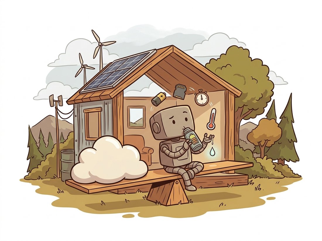
A conservation group deployed camera traps to count animals at remote waterholes with no power and no network. Each trap had a solar panel, a small battery, and a Jetson Orin Nano, and the constraint was brutal: the system had to run a detector on every motion-triggered frame and survive a week of cloudy weather on the battery alone. Their first attempt ran a full YOLO model in FP32 and drained the battery in two days. The team re-budgeted around energy per inference rather than frames per second. They switched to a small YOLO variant, applied int8 quantization with a calibration set built from the traps' own night-vision footage (the calibration distribution matters, as Section 28.1 warned), built an int8 TensorRT engine, and set the Jetson to a low nvpmodel power mode that capped the GPU clock. Inference dropped from 410 mJ to 70 mJ per frame, the trap ran for nine days through overcast weather, and the detector still recovered 94 percent of the animals the FP32 model found. The lesson: at the true edge, the design metric was joules per detection, not milliseconds, and once they optimized the right metric the system became deployable. The accuracy they "lost" to quantization was cheaper than the deployments they lost to dead batteries.
4. Vision on a Phone Intermediate
Phones are the largest edge fleet on earth, and they do not run CUDA. Each mobile platform has its own accelerator (Apple's Neural Engine, Qualcomm's Hexagon, Google's Tensor) and its own runtime to reach it. The three that matter are Core ML on Apple devices, TensorFlow Lite (now LiteRT) on Android and cross-platform, and ExecuTorch, PyTorch's 2024-onward on-device runtime that runs exported PyTorch models on phones and embedded targets directly. All three consume a converted model (Core ML from coremltools, TFLite from a converter, ExecuTorch from torch.export) and dispatch it to whatever accelerator the device has, falling back to the CPU when an operator is unsupported. The conversion to Core ML is representative.
import torch, coremltools as ct
from torchvision.models import mobilenet_v3_small, MobileNet_V3_Small_Weights

model = mobilenet_v3_small(weights=MobileNet_V3_Small_Weights.DEFAULT).eval()
example = torch.randn(1, 3, 224, 224)
traced = torch.jit.trace(model, example)      # Core ML converts a traced graph

# Convert to a Core ML package, quantizing weights to 8 bits during conversion.
mlmodel = ct.convert(
    traced,
    inputs=[ct.ImageType(name="image", shape=example.shape,
                         scale=1/255.0)],      # fold the /255 normalization into the model
    compute_units=ct.ComputeUnit.ALL,          # CPU + GPU + Neural Engine
    minimum_deployment_target=ct.target.iOS17,
)
# Post-training 8-bit weight quantization for a 4x smaller .mlpackage.
mlmodel = ct.optimize.coreml.linear_quantize_weights(mlmodel)
mlmodel.save("MobileNetV3.mlpackage")
print("saved Core ML model; runs on the Neural Engine on supported devices")coremltools, folding the /255 input normalization into the model and quantizing weights to 8 bits. compute_units=ALL lets the runtime place layers on the Neural Engine, GPU, or CPU; the engine chooses per layer at load time. Folding preprocessing into the model graph removes a class of bugs where the app and the model disagree on normalization, an edge echo of the export-validation discipline from Section 28.2.Two practical points recur across all mobile runtimes. First, preprocessing belongs in the graph where possible: the resize, the channel order, and the normalization that the model expects must match exactly what the camera pipeline of Chapter 1 produces, and the safest way to guarantee that is to bake the normalization into the model as above. Second, operator coverage is the real constraint: a mobile accelerator runs a fixed set of operators fast, and a single unsupported operator forces a slow CPU fallback for that layer or a costly accelerator-to-CPU-and-back transfer. Choosing an architecture whose operators the target accelerator supports is often more important than shaving a few FLOPs. Table 28.3.1 summarizes the mobile runtime landscape.
| Runtime | Platform | Accelerator reached | Converted from |
|---|---|---|---|
| Core ML | Apple (iOS, macOS) | Neural Engine, GPU, CPU | coremltools (traced PyTorch) |
| TensorFlow Lite / LiteRT | Android, cross-platform | NNAPI, GPU, Hexagon, CPU | TFLite converter (or via ONNX) |
| ExecuTorch | iOS, Android, embedded | Vendor backends + CPU | torch.export (PyTorch native) |
| ONNX Runtime Mobile | Cross-platform | Core ML / NNAPI providers | ONNX |
The edge is no longer limited to small classifiers. Apple's 2024 on-device foundation models and the 2024-2025 wave of mobile vision-language models (compact variants of the models from Chapter 25) run multi-billion-parameter networks on phones by combining 4-bit weight quantization, the architectural efficiency of this section, and dedicated neural accelerators. The 2023-onward MobileSAM (Zhang et al. 2023, arXiv:2306.14289) and EfficientSAM distilled the promptable segmentation of Chapter 24 into models small enough for real-time on-device use, and the 2023-2024 family of efficient ViTs (EfficientViT; FastViT, Vasu et al. 2023, arXiv:2303.14189) brought transformer accuracy to mobile latency. ExecuTorch's rapid 2024-2025 maturation matters strategically: it lets a model exported with the same torch.export path as the server deployment run natively on the phone, collapsing the training-to-mobile gap that previously required a separate conversion toolchain per platform. The open question for 2026 is how much of a multimodal assistant can run entirely on-device versus split between phone and cloud.
The portrait-mode blur on a modern phone camera is a small segmentation model running in real time on the neural accelerator, separating you from the background frame by frame. The face unlock is a depth-and-recognition pipeline. The photo library that finds every picture of your dog is an on-device classifier and embedding model indexing your library while the phone charges overnight. None of these send your pixels to a server, and none of them existed before the architectures and runtimes of this section made multi-watt vision fit in a pocket. The most widely deployed computer vision on earth is the kind you never notice running.
5. Summary and the Road to Serving
The edge replaces the cloud's single accuracy-and-latency goal with a four-way budget: latency, memory, power, and thermal headroom, measured under sustained load rather than a cold peak. Architectures built for the edge, the depthwise-separable convolution of MobileNet and the compound scaling of EfficientNet, deliver far more accuracy per FLOP than compressing a heavy model down. The Jetson family brings full CUDA and TensorRT compute into a small power envelope, so the export pipeline of Section 28.2 transfers directly; phones reach their accelerators through Core ML, TensorFlow Lite, and the PyTorch-native ExecuTorch, where preprocessing belongs in the graph and operator coverage is the binding constraint. Not every model deploys to a device, though; many live behind an API serving many clients at once. Section 28.4 turns to that world, where the question is not joules per inference but requests per second under a latency target.
On the edge, intermediate activation memory often exceeds weight memory, which is why the inverted-residual block keeps its residual connection across the narrow (projected) ends rather than the wide (expanded) middle. Explain in two or three sentences why a residual stored at the narrow ends uses far less memory than one stored at the expanded middle, and why this matters more on a device with megabytes of RAM than on a server with gigabytes. Connect your reasoning to the activation-memory cost of the feature maps in the CNNs of Chapter 19.
Using the DepthwiseSeparableConv from subsection 2, build two small classifiers identical except that one uses standard convolutions and the other uses depthwise-separable ones, matched as closely as possible in output channels. Count parameters and measure CPU inference latency for both at $224 \times 224$ input. Then train both briefly on CIFAR-10 and record accuracy. Tabulate parameters, latency, and accuracy, and write one paragraph on whether the separable version's efficiency gain came at a measurable accuracy cost for this task, and how that would change your choice for a phone deployment.
Reread the wildlife camera-trap Practical Example. You are given a battery of 50 watt-hours, a solar panel that supplies an average of 8 watt-hours per day, and a requirement to process 2,000 motion-triggered frames per day with a target of surviving 7 cloudy days. Compute the daily energy budget, the maximum energy per inference that meets it, and whether the 70 mJ-per-frame quantized model fits with margin. Then analyze how the budget changes if motion triggers double during migration season, and argue for one design change (model size, power mode, or duty cycle) to absorb it. Justify every number.